Persistent Monitoring of Dynamic Environments
Background:
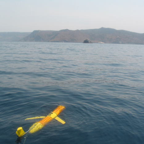
There are some tasks in real world that require to use a sensing robot to estimate field in a dynamic environment. The dynamic field can be ocean temperature, dust accumulation, forest density, oil and nuclear leakage and so on, see Figure 1. But the sensor usually has limited sensing range and the environment is huge. This requires the robot to move around in the environment and motivates the need to plan trajectories for the sensing agent. A trajectory, along which the robot can gather more information and minimize the uncertainties, is preferred to other trajectories.
Research Goal:
Planning trajectories for a sensing robot to estimate field as accurate as possible in a dynamic environment, that is, balance estimation uncertainties in space and time.

Method:
Kalman filter is used to estimate the field. Path planning algorithms are used to plan trajectories to control the evolution of the estimation error covariance matrix.
Method 1:
Based on sampling-based motion planning algorithms, like RRT and RRT*, we proposed one randomized algorithm called Rapidly-exploring Random Cycles (RRC), see video below.
Unlike RRT and RRT*, which return a path between two points, RRC returns a cycle in its environment. It maintains a tree structure, but memorize the best cycle if adding one edge to the tree.
When the sensing robot moves around in the dynamic environment along RRC trajectory, how estimation uncertainties change is given below.
Red curve: trajectory returned by RRC. Yellow circle: a sensing robot. Black blocks: obstacles. The colormap represents the estimation uncertainties of the field over the whole environment. Red hot stands for high uncertainty while dark blue stands for low uncertainty. The points in the same contour line have the same estimation uncertainties.
An experiment using computer to control an m3pi robot to execute the trajectory in a motion capture system (OptiTrack) is given below.
We project the environment on the ground. The robot moves around in the environment, takes measurements and tries to minimize the estimation uncertainties everywhere in the environment. We simulate the measurement process by using motion capture system (OptiTrack) to get the position of the robot and use the position data to update the evolution of the covariance matrix, that is, update the estimation uncertainties in the whole environment, which are represented by colormap.
Method 2:
We use kinodynamic RRT* algorithm to plan trajectories for persistent monitoring problem, see video below.
Kinodynamic RRT* returns a trajectory in a fixed finite time horizon.
When the sensing robot moves around in the dynamic environment along kinodynamic RRT* trajectory, how estimation uncertainties change is given below.
Red curve: trajectory returned by kinodynamic RRT*. Yellow circle: a sensing robot. Black blocks: obstacles. The colormap represents the estimation uncertainties of the field over the whole environment. Red hot stands for high uncertainty while dark blue stands for low uncertainty. The points in the same contour line have the same estimation uncertainties.
An experiment using computer to control an m3pi robot to execute the trajectory in a motion capture system (OptiTrack) is given below.
We project the environment on the ground. The robot moves around in the environment, takes measurements and tries to minimize the estimation uncertainties everywhere in the environment. We simulate the measurement process by using motion capture system (OptiTrack) to get the position of the robot and use the position data to update the evolution of the covariance matrix, that is, update the estimation uncertainties in the whole environment, which are represented by colormap.
Method 3:
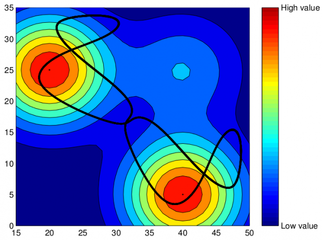
We use optimal control technique (Matrix Minimum Principle) to find trajectories for agents doing persistent monitoring.
An example trajectory is given in Figure 3.

When the sensing robot moves around in the dynamic environment along a trajectory, how estimation uncertainties change is given below.
Black curve: trajectory returned by solving a set of differential equations given by Matrix Minimum Principle. Yellow circle: a sensing robot. The colormap represents the estimation uncertainties of the field over the whole environment. Red hot stands for high uncertainty while dark blue stands for low uncertainty. The points in the same contour line have the same estimation uncertainties.